Math Methods for Gaussian Distribution

Gaussian (Normal) Distribution

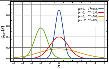
If the probability distribution of X is Gaussian^ (aka Normal) with mean (µ or mu) and variance sigma squared (ó² or sigma2) we write X ~ N(µ, ó²). {ed, using ó as the greek letter sigma}. µ gives us the center of the normal bell curve, ó is the standard deviation^ or width from the center of the curve to the inflection point^ where the slope of the curve changes from concave to convex. ó² is the variance.

In the figure here, the red line is the Normal distribution.

Another way of calculating this is:

ó²=o^2 a = 1/sqrt(2 * Pi *ó²)

g(x) = a * exp(-0.5 * ( (x-µ)^2 /ó²) )

Where ó² is the variance which controls the width of the peak, µ is the "expected value" or position of the center of the peak, and a is the height of the peak. Setting a to 1/sqrt(2* Pi *ó²) makes the integral of the curve exactly 1, so the area under the curve is a single unit.

Gausian functions are often used as kernels in Support Vector Machines, or in Anomaly Detection. They are also used in Kalman Filters for localization

Pascal / Delphi program RandomGaussianSD1 returns a number drawn from a Gaussian distribution with mean of zero, unit standard deviation, cutoff at +/- 4

Random Gaussian Variables